Sci-fi Primers: Remote Sensing - Part 6
A deeper dive into to the maths and science of remote sensing

Finally, we’re going to take a deeper dive into to the maths and science behind remote sensing.
Electromagnetic Radiation
Frequency and wavelength
Electromagnetic radiation travels at the speed of light c when in vacuum, defined exactly as 299,792,458 metres/second (around 300,000 kilometres/second). A given signal will have a frequency f and wavelength w. Frequency is the number of full waves per second, while the wavelength is the physical distance between two consecutive waves. The two are related by formula
This reads: the speed of light is equal to the frequency multiplied by the wavelength. As the speed of light stays fixed, an increase in frequency leads to a proportional decrease in wavelength, e.g., doubling the frequency will half the wavelength.
This means that very low frequency signals like radio waves have very long wavelengths (often many kilometres long), while higher frequency signals like visible light have wavelengths on the sub-micron scale.
Details on the Spectrum
We discuss the frequency and wavelength to highlight an important aspect of electromagnetic radiation: it interacts with matter very differently at different frequencies and wavelengths.
Namely, it interacts with physical structures similar in size to its own wavelength.
An example: X-rays have a wavelength on the nanometre scale, which is around the size of the space between molecules. This allows scientists to use something called X-ray crystallography to probe the molecular structure. However, using another part of the spectrum wouldn’t work for this purpose, because those parts of the spectrum correspond to wavelengths much smaller or larger than the space between atoms.
Optical Limits
Practical Resolving Power of Telescope (Dawes Limit)
There are many factors that influence the upper limit of what can be seen with a given telescope. William Dawes condensed all this into a simple equation to express the practical limit for classical telescopes:
where R is the resolving power in arcseconds (1/3600th of a degree) and D is the diameter of the main lens in centimetres.
Arc is the standard unit of angle in astronomy, rather than degrees, so this may be unfamiliar. But you can easily convert between them like so:
A worked example: using the equation above, we calculate that a telescope with a main lens 1 metre across will have a resolving power of 0.12 arcseconds. Assuming your telescope is in orbit around the Earth, and you want to be able to clearly see a fleet of spaceships, each of which are 1 kilometre across. How far away can they be before they start to blur together?
We need to use a bit of trigonometry here:
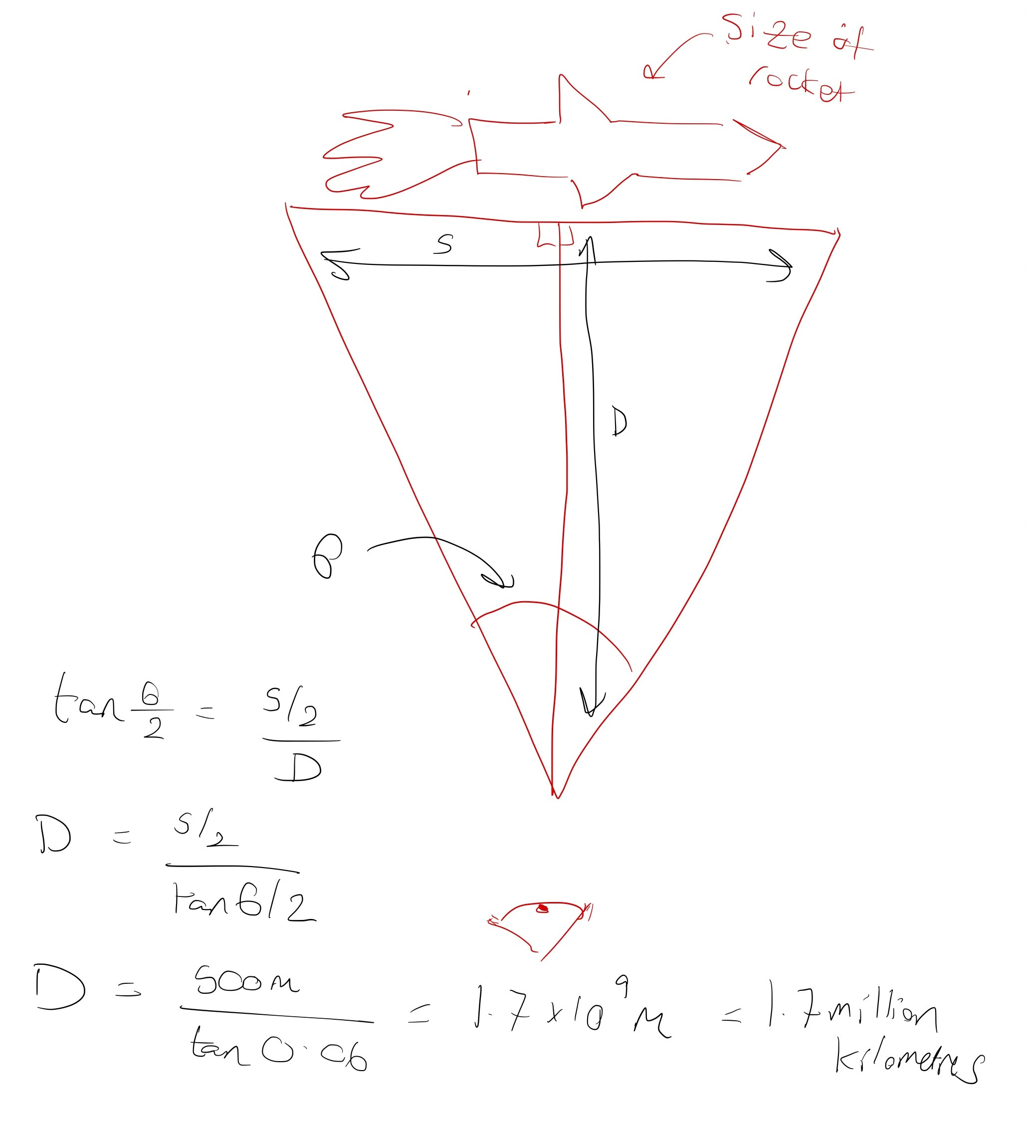
Our workings here say S = 1 kilometre, so S/2 = 500 metres, and the resolving angle theta is our 0.012 arcseconds, and so theta/2 = 0.06 arcseconds. Crunching the numbers, the distance between the observer and the target can be maximum of 1.7 million kilometres. For reference, the distance between the Earth and Mars is 225 million kilometres, so to see a 1 kilometre-wide target on Mars, you’re going to need a much bigger telescope. But, the distance between the Earth and the Moon is 384,400 kilometres, so we can see things significantly smaller than 1 kilometres from Earth.
Definition of Information
Information in the formal sense is difficult to define, and this field goes off in all sorts of odd tangents (including an intricate association with entropy). We’ll try to stick the most pertinent aspects.
The information content of an event H is expressed in terms of the probability p that an event E will happen:
We we have the equation graphed below:
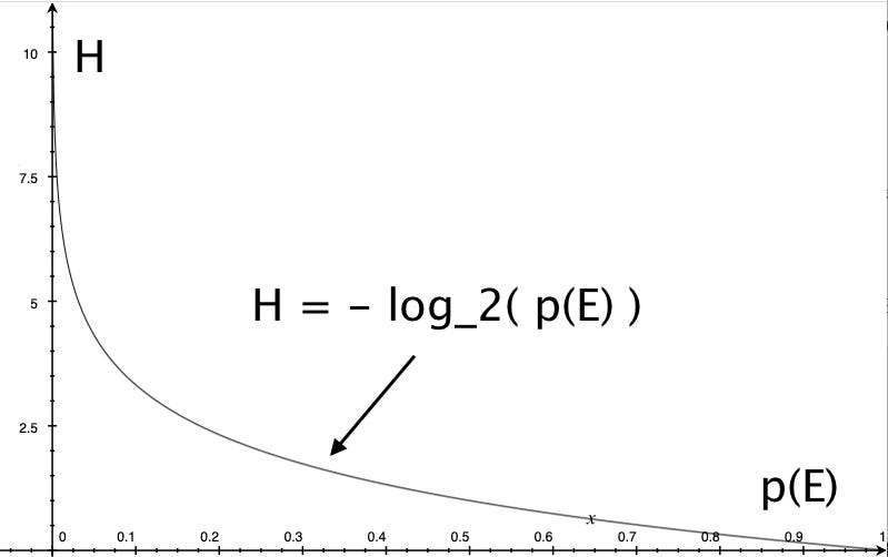
The results might seem counterintuitive. A high-probability event has less information.
This can be understood by thinking of information as how surprising a given received signal would be. A high probability event, like the usual crackle of static you’re always hearing if nothing is being transmitted, carries no useful information. However, hearing a message that spells out tomorrow’s winning lottery numbers contains information of an event very unlikely to happen, and so is an observation worth paying attention to.
Data Rate Constraints
The Shannon-Hartley Theorem
Transmitting data over any channel has limits, especially due to inevitable noise competing with the signal. The Shannon-Hartley theorem expresses the maximum transmittable information-rate C in bits/second as:
Where S/N is the signal-to-noise ratio, and B is the bandwidth in Hz (the range of frequencies to transmit over).
The signal-to-noise ratio is the strength of the signal you’re trying to send divided by the strength of the background noise. For example, the below we can graph information-rate (vertical axis) for increasing signal-to-noise ratio (horizontal axis), assuming a bandwidth of 20 MHz (typical for a 2.5 GHz wifi channel):
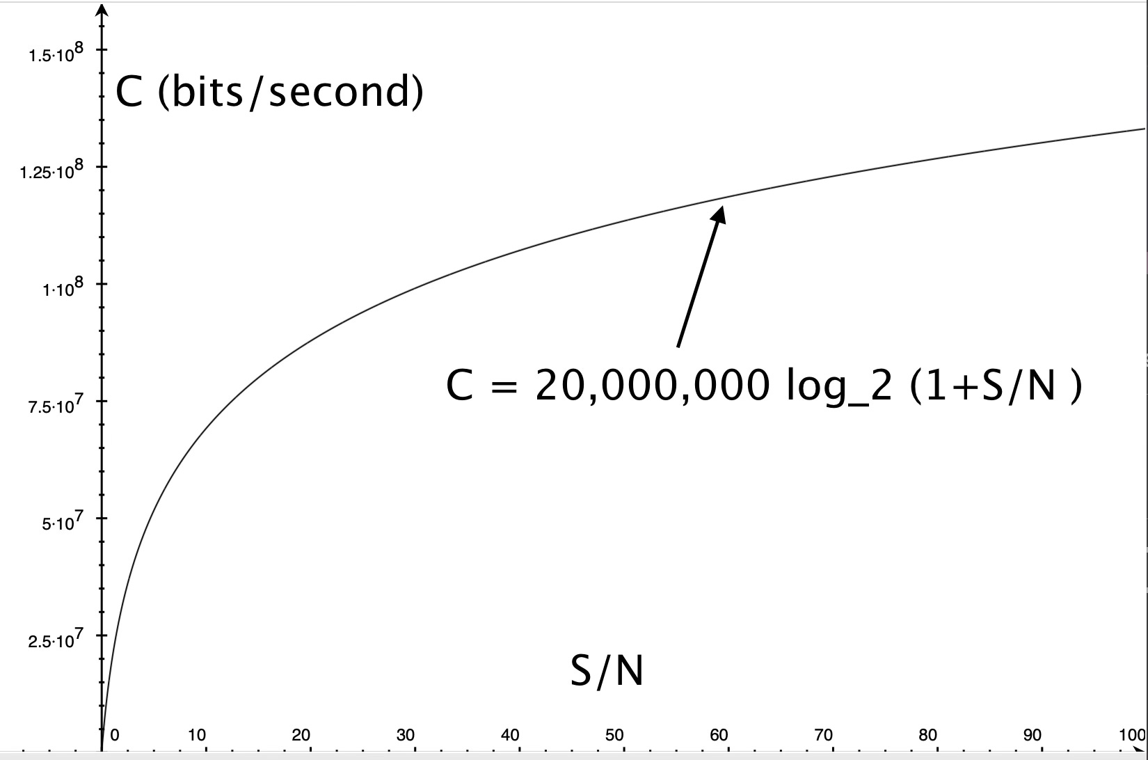
We can see that when S/N = 100 (our signal is a hundred times stronger than the background noise), we can get a maximum of around 120,500,000 bits/second through the channel, or around 120 Megabits/second.
What we see here is the theoretical limit of the effect of somebody “boosting the power of the signal”.
That concludes the primer on remote sensing. Watch out for more soon!